Discover Pandipedia

Introduction to Variational Lossy Autoencoders

Variational autoencoders (VAEs) are a powerful class of generative models that are designed to learn representations of data in a way that is amenable to downstream tasks like classification. However, the introduction of a new method called Variational Lossy Autoencoder (VLAE) offers a novel perspective by leveraging the concept of lossy encoding to improve representation learning and density estimation.

What is a Variational Lossy Autoencoder?

The core idea behind a VLAE is to combine the strengths of variational inference with the lossy encoding properties of certain types of autoencoders. In essence, traditional VAEs aim to reconstruct data as accurately as possible, often leading to overly complex representations that capture noise rather than relevant features. In contrast, VLAEs intentionally embrace a lossy approach, aiming to retain the essential structure of the data while discarding unnecessary details. This is particularly useful when considering high-dimensional data, such as images, where the goal is not always precise reconstruction but rather capturing the most relevant information^[1].

Representation Learning and Density Estimation

VLAEs facilitate representation learning by focusing on the components of the data that are most salient for downstream tasks. For instance, a good representation can be essential for image classification, where capturing the overall shape and visual structure is often more important than faithfully reconstructing each pixel^[1].

The authors propose a method that integrates autoregressive models with VAEs, enhancing generative modeling performance. By explicitly controlling what information is retained or discarded, VLAEs can potentially achieve better performance on various tasks compared to traditional VAEs, which tend to preserve too much data^[1].

Mechanism of Variational Lossy Autoencoders

In a typical VLAE setup, the model incorporates a global latent code along with an autogressive decoder which models the conditional distribution of the data^[1]. This approach helps in efficiently utilizing the latent variable framework. The authors note that previous applications of VAEs often neglected the latent variables, which led to suboptimal representations. By using a simple yet effective decoding strategy, VLAEs can ensure that learned representations are both efficient and informative, striking a balance between accuracy and complexity^[1].

Technical Background

The architecture of a VLAE generally builds upon traditional VAE models but introduces innovations to address the shortcomings of standard approaches. For example, the model can be structured to ensure that certain aspects of information are retained while others are discarded, facilitating a better understanding of how to learn from data without overfitting to noise. The VLAE also leverages sophisticated statistical techniques to optimize its variational inference mechanism, making it a versatile tool in the generative modeling arsenal^[1].

Results and Application

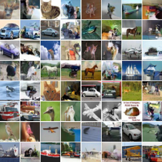
Experimental results from applying VLAEs to datasets like MNIST and CIFAR-10 demonstrate promising outcomes. For instance, when employing VLAEs on binarized MNIST, the model outperformed conventional VAEs by using an AF prior instead of the IAF posterior, highlighting its ability to learn nuanced representations without losing critical information. The authors present statistical evidence showing that VLAEs achieve state-of-the-art results across various benchmarks^[1].

Lossy Compression Demonstrated

The authors emphasize the effectiveness of VLAEs in compression tasks. By focusing on lossy representations, the VLAE is capable of generating high-quality reconstructions that retain meaningful features while disregarding less relevant data. In experiments, the lossy codes generated by VLAEs were shown to maintain consistency with the original data structure, suggesting that even in a lossy context, useful information can still be preserved^[1].

Comparison with Traditional VAEs

A notable distinction between VLAEs and traditional VAEs lies in their approach to latent variables. In traditional VAEs, the latent space is usually optimized for exact reconstruction. In contrast, VLAEs allow for a more flexible interpretation of the latent variables, encouraging the model to adaptively determine the importance of certain features based on the task at hand, rather than strictly interpreting all latent codes as equally important^[1].

This flexibility in VLAEs not only enhances their performance for specific tasks like classification but also improves their capabilities in more general applications, such as anomaly detection and generative art, where the preservation of structural integrity is crucial^[1].

Conclusion

Variational Lossy Autoencoders represent a significant advancement in the field of generative modeling. By prioritizing the learning of structured representations and embracing lossy encoding, VLAEs provide a promising pathway for improved performance in various machine learning tasks. The integration of autoregressive models with traditional VAEs not only refines the representation learning process but also enhances density estimation capabilities. As models continue to evolve, VLAEs stand out as a compelling option for researchers and practitioners looking to leverage the strengths of variational inference in practical applications^[1].

Introduction to GPipe

The paper titled 'GPipe: Easy Scaling with Micro-Batch Pipeline Parallelism' introduces a novel method for efficiently training large neural networks. The increasing complexity of deep learning models has made optimizing their performance critical, especially as they often exceed the memory limits of single accelerators. GPipe addresses these challenges by enabling effective model parallelism and improving resource utilization without sacrificing performance.

Pipeline Parallelism Explained

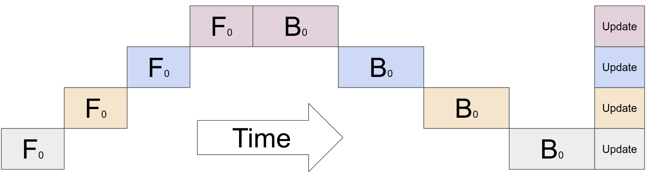
Scaling deep learning models typically requires distributing the workload across multiple hardware accelerators. GPipe specifically focuses on pipeline parallelism, where a neural network is constructed as a sequence of layers, allowing for parts of the model to be processed simultaneously on different accelerators. This approach helps in handling larger models by breaking them into smaller sub-parts, thus allowing each accelerator to work on a segment of the model, increasing throughput significantly.

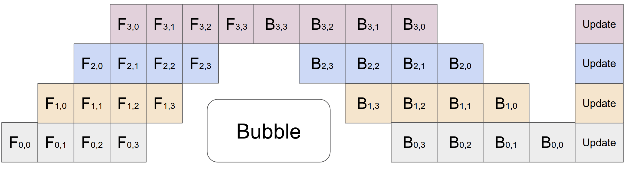
The authors argue that by utilizing 'micro-batch pipeline parallelism,' GPipe enhances efficiency by splitting each mini-batch into smaller segments called micro-batches. Each accelerator receives one micro-batch and processes it independently, which helps facilitate better hardware utilization compared to traditional methods that may lead to idle processing times on some accelerators due to sequential dependencies between layers^[1].

Advantages of Using GPipe

Improved Training Efficiency

GPipe not only maximizes the capacity of large-scale models but also provides substantial improvements in training speed. The paper reports that using GPipe with various architectures yields significant speedups when scaling the number of accelerators. For example, when training an AmoebaNet model, the authors noted that scaling to 8 accelerators enhanced the training efficiency multiple times compared to non-pipelined approaches^[1].

Flexibility in Model Structures

One of the standout features of GPipe is its adaptability to various model architectures, such as convolutional neural networks and transformers. GPipe supports different layer configurations and can dynamically adjust to the specific needs of a given architecture. This flexibility provides researchers and practitioners with the tools they need to optimize models for diverse tasks, including image classification and multilingual machine translation, as demonstrated through their experiments on large datasets^[1].

Experiments and Findings

Through extensive experiments, the authors demonstrate that GPipe can effectively scale large neural networks. They utilized various architectures—including the 557-million-parameter AmoebaNet and a 1.3B-parameter multilingual transformer model—across different datasets like ImageNet and various translation tasks.

The results showed that models trained with GPipe achieved higher accuracy and better performance metrics, such as BLEU scores in translation tasks, compared to traditional single-device training methods. Specifically, they achieved a top-1 accuracy of 84.4% on ImageNet, showcasing the potential of deeper architectures paired with pipeline parallelism^[1].

Addressing Performance Bottlenecks

The design of GPipe counters several potential performance bottlenecks inherent in other parallel processing strategies. One major challenge is the communication overhead between accelerators, particularly in synchronizing the gradient updates. GPipe introduces a novel back-splitting technique that minimizes this overhead by allowing gradients to be computed in parallel while ensuring they are updated synchronously at the end of each training iteration. This allows for seamless integration across multiple devices, significantly reducing latency and maximizing throughput^[1].

Practical Implementation Considerations

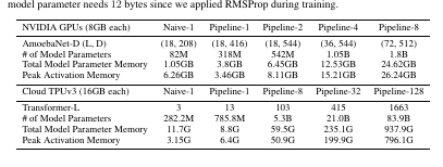
Implementing GPipe requires considerations around factors like memory consumption. The paper discusses how re-materialization, during which activations are recomputed instead of stored, can significantly reduce memory overhead during training. This is particularly beneficial when handling large models that otherwise might not fit into the available capacity of a single accelerator. By applying this strategy, GPipe can manage larger architectures and ensure efficient resource allocation across the various components involved in training^[1].

Conclusion

GPipe represents a significant advancement in the training of large-scale neural networks by introducing pipeline parallelism combined with micro-batching. This innovative framework allows for efficient model scaling while maintaining training performance across different architectures. The approach not only enhances scalability but also provides a flexible and robust solution for tackling modern deep learning challenges efficiently. Researchers and engineers can leverage GPipe to optimize their training regimes, making it a valuable tool in the ever-evolving landscape of artificial intelligence^[1].

Introduction

Deep Residual Networks (ResNets) have revolutionized the way we construct and train deep neural networks. They tackle the problem of vanishing gradients in neural networks by introducing skip connections, allowing gradients to flow more easily and enabling the training of very deep models. This blog post synthesizes findings from the paper 'Identity Mappings in Deep Residual Networks' to highlight key innovations and implications in deep learning architecture.

Background on Residual Networks

Residual Networks utilize a fundamental building block called a 'Residual Unit.' The basic formulation of a Residual Unit is represented as:

[ y_l = h(x_l) + F(x_l, W_l) ]
[ x_{l+1} = F(y_l) ]

Where ( x_l ) is the input, ( h(x_l) ) is an identity mapping, and ( F(x_l, W_l) ) represents the residual function with weights ( W_l ). This design allows a direct path for the signal to travel through layers, supporting both forward and backward propagations effectively, which is critical for optimizing deep networks^[1].

The Role of Identity Mappings

The core concept in this research emphasizes the importance of identity mappings within residual units. The paper argues that if ( F ) behaves like an identity mapping, the gradient ¬can propagate seamlessly. This is essential, as it allows the deeper layers to train effectively without suffering from vanishing gradient issues. The authors propose modifications to traditional ResNet architectures to better capture these identity mappings, resulting in improved performance on various tasks^[1].

Experimental Insights

The research presents extensive experiments, particularly using the CIFAR-10 dataset, which indicate that certain architectures facilitate easier optimization and lower error rates. One notable observation is that deeper networks, like the 110-layer ResNet, showcase significant error reduction when identity mappings are integrated optimally, enhancing performance by preventing overfitting and alleviating the challenges of training deep networks^[1].

Effects of Activation Functions

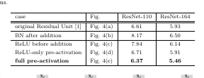
An important aspect discussed in the paper is the influence of activation functions on the performance of residual networks. Traditional designs often use ReLU (Rectified Linear Unit) activation post addition. However, this can lead to suboptimal situations where the output can become very negative or the gradient diminishes. Instead, the authors explore the concept of using activation functions before addition, referred to as 'pre-activation.' This architectural change results in consistently lower error rates across various networks, suggesting better representation capabilities and optimization efficiency^[1].

Various Shortcut Connections

The research also investigates different types of shortcut connections in Residual Units. These include constant scaling, exclusive gating, and dropout shortcuts. The findings illustrate that while simpler shortcuts like the identity mapping are effective, more complex gating mechanisms do not consistently yield performance improvements. Instead, they may hinder learning in deep networks due to the added complexity^[1].

Performance Metrics

In their experiments, the authors provide detailed comparisons across several models, emphasizing the following key findings:

• The original Residual Unit offers competitive performance, showing a significant lead over simpler architectures.

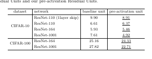
• The 'pre-activation' model consistently outperforms traditional designs across various datasets, including CIFAR-10 and CIFAR-100, achieving lower error rates and demonstrating better training convergence characteristics^[1].

Conclusion

The insights from 'Identity Mappings in Deep Residual Networks' underline the centrality of identity mappings and the innovative design of residual units in enhancing deep learning architectures. By allowing gradients to flow unhindered, they enable deeper networks to learn more effectively and achieve better performance.

The exploration of activation functions and shortcut connections expands our understanding of how different architectural choices can significantly impact the learning and convergence of deep neural networks. This work not only enriches theoretical foundations but also provides practical guidelines for designing efficient deep learning models in various applications, paving the way for future advancements in the field of artificial intelligence and machine learning^[1].

Introduction to the Research

In a groundbreaking study, researchers Alex Krizhevsky, Ilya Sutskever, and Geoffrey Hinton trained a deep convolutional neural network (CNN) to classify over 1.2 million high-resolution images from the ImageNet database, spanning 1,000 different categories. Their work significantly advanced image classification accuracy, achieving a top-1 error rate of 37.5% and a top-5 error rate of 17.0%, outperforming previous state-of-the-art methods by a notable margin^[1].

The Neural Network Architecture

The architecture of the developed CNN is complex, consisting of five convolutional layers followed by three fully-connected layers. The model includes more than 60 million parameters, making it one of the largest neural networks trained on ImageNet at the time. To maximize training efficiency, the researchers employed GPU implementation of 2D convolution and innovative techniques like dropout to reduce overfitting^[1].

The architecture can be summarized as follows:

• Convolutional Layers: These layers extract features from the input images, helping the network learn patterns essential for classification.

• Max Pooling Layers: These are used to reduce the spatial dimensions of the feature maps, retaining essential information while reducing computational load^[1].

• Fully-Connected Layers: They integrate the features learned in the convolutional layers to produce the final classification output.

Training and Regularization Techniques

To optimize the network's performance and prevent overfitting, several effective strategies were implemented during training:

1. Data Augmentation: The researchers expanded the training dataset using random 224x224 pixel patches and horizontal reflections, enhancing the model's ability to generalize from limited data^[1].

2. Dropout: This novel technique involved randomly setting a portion of hidden neurons to zero during training. By doing so, the network learned to rely on various subsets of neurons, improving robustness and reducing overfitting^[1].

3. Local Response Normalization: This process helps to enhance feature representation by normalizing the response of the neurons, aiding in better generalization during training^[1].

Results and Performance

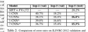
The deep CNN achieved remarkable results in classification tasks, demonstrating that using a network of this size could lead to unprecedented accuracies in image processing. In the ILSVRC-2012 competition, they fine-tuned their model to classify the entire ImageNet 2011 validation set, obtaining an error rate of 15.3%. This performance was significantly better than other competing models, which achieved a top-5 error rate of 26.2%^[1].

The researchers also noted the importance of the model's depth. They observed that reducing the number of convolutional layers negatively impacted performance, illustrating the significance of a deeper architecture for improved accuracy^[1].

Visual Insights from the Model

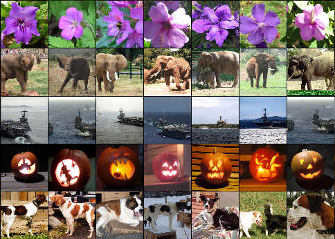
To qualitatively evaluate the CNN's performance, images from the test set were examined based on top-5 predictions. The model often recognized off-center objects accurately. However, there was some ambiguity with certain images, indicating that additional training with more variable datasets could enhance accuracy further^[1].

An interesting observation from their analysis was how the trained model could retrieve similar images based on feature vectors. By using the Euclidean distance between feature vectors, the researchers could identify related images, demonstrating the model's understanding of visual similarities^[1].

Future Directions

While the results showcased the capabilities of deep learning in image classification, the authors acknowledged that the network's performance could further improve with more extensive training and architectural refinements. They hinted at the potential for future work to explore different architectures and training datasets to enhance model performance^[1].

Additionally, as advancements in computational power and methodologies continue, larger architectures may become feasible, enabling even deeper networks for more complex image classification tasks^[1].

Conclusion

The study on deep convolutional neural networks for ImageNet classification represents a significant milestone in the field of computer vision. By effectively combining strategies like dropout, data augmentation, and advanced training methods, the researchers set new standards for performance in image classification tasks. This research not only highlights the potential of deep learning but also opens doors for future innovations in artificial intelligence and machine learning applications^[1].